From live traffic feeds to a history I could query.
I built a collector, a database, and a dashboard to explore Luxembourg’s traffic over time. The work was as much about preserving the evidence as drawing the charts.
The CITA feeds describe the latest road conditions. To compare hours, days, or roads later, I needed to collect those changing states myself. Seven measurement feeds sit alongside incidents, regulations, and static and dynamic parking data, each with its own structure and update rhythm.
I separated the collector from the dashboard. The collector keeps building the history while the interface is closed, and the dashboard can query stored observations when a feed is unavailable.
Inside the engineering
Follow a response through the system.
Each stage has a specific responsibility. Keeping those boundaries clear let me trace a result back through the query, parser, and original response.
Open a stage to inspect the decision and its consequences.
Each feed has its own schedule: incidents every minute, measurements and dynamic parking every five minutes, regulations every fifteen minutes, and static parking once a day. A single scheduler processes due feeds sequentially, with bounded retries and timeouts.
Before parsing, I hash the response bytes with SHA-256 and preserve new contents as gzip files. A temporary file, fsync, and an atomic rename protect the archive write.
Why this order matters
A parser can fail without destroying the input that explains the failure. If the database is unavailable, the collector still attempts filesystem archival.
02Identify · SHA-256Keep the fetch. Reuse the content.Repeated bytes → one snapshot, another observation+
Two byte-identical responses from the same feed share one snapshot. Every fetch still gets its own observation, so the history records when unchanged content was delivered again. The collector skips parsing a registered duplicate.
When the response is a duplicate
if duplicate:
    return FeedCollectionResult(
        feed.name, snapshot_id,
        archived.sha256,
        archived.path,
        duplicate=True
    )
collector/collector.py · collect_feed Excerpt, with line breaks adjusted. Snapshot registration has already recorded the fetch; the early return skips parsing.
Measured in the evaluation
49,488 fetches returned known content. Hashing detects byte equality; differently formatted XML can still describe the same information without sharing a hash.
03Parse · DATEX IIHandle each feed on its own terms.XML → domain objects and structured warnings+
Feed-specific parsers handle the different DATEX II structures, namespaces, nested records, and optional values. Missing values remain missing; an unknown coordinate system is preserved with a warning rather than guessed onto a map.
When parsing has failed
if snapshot_id is not None:
    mark_snapshot_failed(
        snapshot_id,
        exc,
        database_url
    )
collector/collector.py · collect_feed Exception-handler excerpt, with line breaks adjusted. The snapshot is marked as failed; its already archived response remains available.
A recoverable input
The evaluation recorded 46 failed parses. Their raw responses remained available for diagnosis. An offline reprocessing command can apply an updated parser to archived snapshots.
The detailed schema preserves measurements, versioned incident records, regulations, parking data, and their snapshot references. Flatter compatibility tables support the existing historical queries.
The parsed output and its compatibility projection are written in one transaction. A failed write rolls back that group while the archived source remains. Unique keys prevent uncontrolled duplication.
The tradeoff
Raw bytes and relational projections serve different tasks, at the cost of extra storage and consistency work. The evaluation database occupied roughly 15 GB including indexes.
05Query & explore · SQL, Polars, StreamlitAsk the history, not the live feed.Stored measurements → filtered views and comparisons+
PostgreSQL filters and aggregates before results reach Polars and Streamlit. Historical series stay separated by road and stored direction. Timestamps are stored in UTC; hourly and weekday profiles use Europe/Luxembourg.
The dashboard provides current observations, a map, history, comparisons, collection integrity, and data-quality views. Automatic refresh is limited to live areas.
A correction that changed the chart
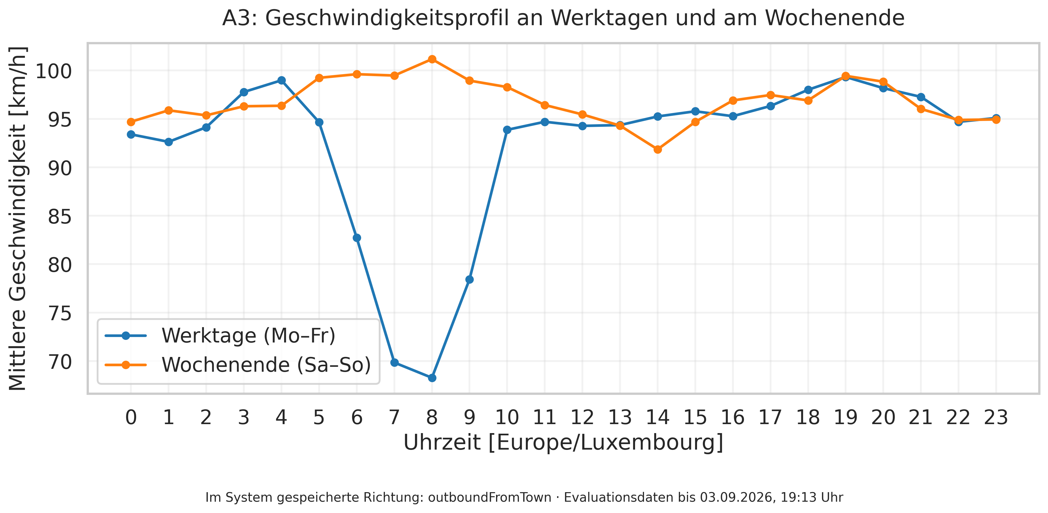
Early charts connected different directions into artificial zigzags. I fixed the series grouping and aggregation rather than smoothing the line.
In my sample, weekday speeds dipped in the morning; the weekend profile stayed steadier.
Weekday vs. weekend mean speeds · A3 · stored direction outboundFromTown
Historical observations
Explore the day Hover or drag to inspect an hour. Keyboard: ← / →, Home / End; Escape resets to 08:00.
Collected 23 July–3 September 2026 · Europe/Luxembourg. Observation-weighted hourly means: Monday–Friday versus Saturday–Sunday. Source: thesis section 6.4.1 / figure 6.4 and its hourly export. All hourly groups have observations; collection gaps remain in the source. Missing hourly values stay as breaks. The stored direction label is not independently verified geographically.Read the data and method +
Source: my bachelor’s thesis, section 6.4.1 / figure 6.4, and its evaluation_hourly_profile.csv export. I grouped Monday–Friday and Saturday–Sunday and weighted each weekday/hour mean by its observation count, following the thesis plotting code. Source rows include positive speed, flow, and occupancy values; results are rounded to 0.1 km/h. The source window runs from 23 July 2026, 16:23 to 3 September 2026, 19:13 (Europe/Luxembourg).
Scroll within the table to see all hours and columns. Speeds are in km/h; observation columns show sample counts.
A3 hourly profile · stored direction outboundFromTown
Hour
Weekday km/h
Observations
Weekend km/h
Observations
00:00
93.4
4,357
94.7
1,731
01:00
92.6
4,236
95.9
1,730
02:00
94.1
4,217
95.4
1,651
03:00
97.8
4,334
96.3
1,644
04:00
99.0
4,404
96.4
1,632
05:00
94.7
4,503
99.2
1,641
06:00
82.7
4,502
99.6
1,645
07:00
69.8
4,580
99.5
1,675
08:00
68.3
4,600
101.2
1,706
09:00
78.4
4,559
99.0
1,645
10:00
93.9
4,540
98.3
1,682
11:00
94.7
4,531
96.4
1,699
12:00
94.3
4,611
95.5
1,726
13:00
94.4
4,543
94.3
1,693
14:00
95.3
4,578
91.9
1,671
15:00
95.8
4,581
94.7
1,685
16:00
95.3
4,614
96.9
1,669
17:00
96.3
4,680
97.5
1,702
18:00
98.0
4,685
96.9
1,662
19:00
99.3
4,500
99.4
1,659
20:00
98.2
4,460
98.8
1,732
21:00
97.3
4,441
96.0
1,751
22:00
94.7
4,364
94.9
1,749
23:00
95.1
4,405
94.9
1,697
Reproduce this result →Start with the public export. No database or university account needed.
High flow alone wasn’t enough.
At 08:00 in the weekday outboundFromTown profile, A3 mean speed was 68.3 km/h at about 2,551 vehicles/hour. A6 carried a higher flow of about 2,921 vehicles/hour while averaging 95.6 km/h.
I therefore considered speed, flow, and occupancy together. This comparison does not establish why the roads differed or rank their capacity.
Thesis §6.5.2 · Figure 6.6
Recurring windows needed more than one hour.
The rule requires speed ≤75 km/h, flow ≥900 vehicles/hour, and occupancy ≥10%, with at least eight observations from three dates per weekday/hour profile. At least two qualifying hours must be consecutive.
Seven windows qualified, all on the A3: mornings in one stored direction and afternoons in the other. These are project-specific rules without external ground-truth validation.
Thesis §6.6 · Table 6.5
Inspect all seven A3 load windows +
Thesis table 6.5 · Europe/Luxembourg. End times are exclusive: 07:00–09:00 includes the hours beginning at 07:00 and 08:00. Values are observation-weighted means. Scroll horizontally on a narrow screen.
Recurring load windows in the archived evaluation sample
Stored direction
Weekday
Local time
Speed km/h
Flow vehicles/h
Occupancy %
outboundFromTown
Monday
07:00–09:00
67.1
2,512
11.8
outboundFromTown
Tuesday
07:00–10:00
67.5
2,476
11.7
outboundFromTown
Wednesday
07:00–09:00
68.6
2,574
11.6
outboundFromTown
Thursday
07:00–09:00
68.7
2,656
11.6
inboundTowardsTown
Monday
15:00–19:00
69.5
2,059
11.2
inboundTowardsTown
Tuesday
16:00–18:00
70.8
2,187
11.0
inboundTowardsTown
Thursday
15:00–18:00
71.8
2,189
11.0
The direction labels are stored categories. Their geographic meanings were not independently verified for every road, so I do not translate them into compass or city-bound directions.
What failed · 25 July 2026
The missing 18 hours, 10 minutes.
A high success rate can hide a long, continuous gap.
The evaluation reported successful outcomes for 98.14% of 161,746 feed-specific collection runs. Yet all seven measurement feeds shared a gap of roughly 18 hours and 10 minutes on 25 July.
Find the shared failure.Around 02:26, successful fetches stopped across all seven roads. Other clients could still connect; the Python client failed during TLS negotiation.
Restore collection.Restricting the shared HTTP client to TLS 1.2 restored successful fetches, around 20:37 local time.
Keep the gap visible.The source did not offer those missed historical observations for retrieval. Collection resumed, but the missing measurements could not be recovered.
Thesis §6.2.3 · Figure 6.1. Success rate is a share of logged runs, not uptime or complete temporal coverage.
What I would improve
Keep the limits as visible as the results.
Verify direction semantics.
About 10% of measurements lacked a normalized direction. The remaining labels still need independent geographic validation.
Version quality assessments.
The dashboard computes quality dynamically. Historical fields remain unassessed; reproducing an earlier judgment needs its rule version and evaluation time.
Finish the alert integration.
Alert candidates, persistence, and lifecycle tests exist. Automatic synchronization was not wired into the main collector or dashboard flow.
Evaluate over a longer period.
43 days support weekly patterns, not seasonal claims. A longer dataset, independent traffic labels, load tests, and user studies would strengthen the evaluation.